Explore this notebook interactively:
Gallery#
In this notebook we show different types of queries and how their response look like.
Content#
Prepare#
Import packages:
[1]:
import semantique as sq
[2]:
import pandas as pd
import geopandas as gpd
import xarray as xr
import matplotlib.pyplot as plt
import numpy as np
import json
import copy
Set the context of query execution.
[3]:
# Load a mapping.
with open("files/mapping.json", "r") as file:
    mapping = sq.mapping.Semantique(json.load(file))

# Represent an EO data cube.
with open("files/layout_gtiff.json", "r") as file:
    dc = sq.datacube.GeotiffArchive(json.load(file), src = "files/layers_gtiff.zip")

# Set the spatio-temporal extent.
space = sq.SpatialExtent(gpd.read_file("files/footprint.geojson"))
time = sq.TemporalExtent("2019-01-01", "2020-12-31")

# Collect the full context.
# Including additional configuration parameters.
context = {
    "datacube": dc,
    "mapping": mapping,
    "space": space,
    "time": time,
    "crs": 3035,
    "tz": "UTC",
    "spatial_resolution": [-10, 10]
}
Count water and vegetation presence#
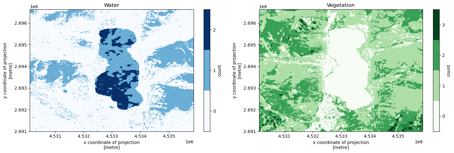
First, we count for each location in our spatial extent how many times during our temporal extent a certain semantic concept (in this example we use water and vegetation) was observed.
Then, we count for each timestamp at which observations were made during our temporal extent at how many locations in our spatial extent these concepts were observed.
[4]:
recipe = sq.QueryRecipe()

recipe["water_count_time"] = sq.entity("water").reduce("count", "time")
recipe["vegetation_count_time"] = sq.entity("vegetation").reduce("count", "time")
recipe["water_count_space"] = sq.entity("water").reduce("count", "space")
recipe["vegetation_count_space"] = sq.entity("vegetation").reduce("count", "space")

response = recipe.execute(**context)
[5]:
f, (ax1, ax2) = plt.subplots(1, 2, figsize = (15, 5))

water_count = response["water_count_time"]
values = list(range(int(np.nanmin(water_count)), int(np.nanmax(water_count)) + 1))
levels = [x - 0.5 for x in values + [max(values) + 1]]
colors = plt.cm.Blues
water_count.plot(ax = ax1, levels = levels, cmap = colors, cbar_kwargs = {"ticks": values, "label": "count"})
ax1.set_title("Water")

vegetation_count = response["vegetation_count_time"]
values = list(range(int(np.nanmin(vegetation_count)), int(np.nanmax(vegetation_count)) + 1))
levels = [x - 0.5 for x in values + [max(values) + 1]]
colors = plt.cm.Greens
vegetation_count.plot(ax = ax2, levels = levels, cmap = colors, cbar_kwargs = {"ticks": values, "label": "count"})
ax2.set_title("Vegetation")

plt.tight_layout()
plt.draw()
[6]:
water_count_df = response["water_count_space"].sq.to_dataframe()
vegetation_count_df = response["vegetation_count_space"].sq.to_dataframe()
water_count_df.join(vegetation_count_df, on = "time")
[6]:
| water_count_space | vegetation_count_space | |
|---|---|---|
| time | ||
| 2019-12-15 10:17:33.408715 | 0.0 | 6045.0 |
| 2020-09-05 10:17:43.167942 | 44804.0 | 243234.0 |
| 2020-12-19 10:17:34.610661 | 78607.0 | 89174.0 |
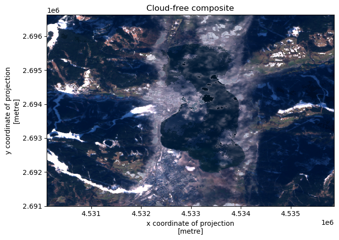
Cloud-free composite#
[7]:
recipe = sq.QueryRecipe()

red_band = sq.reflectance("s2_band04")
green_band = sq.reflectance("s2_band03")
blue_band = sq.reflectance("s2_band02")

recipe["composite"] = sq.collection(red_band, green_band, blue_band).\
    filter(sq.entity("cloud").evaluate("not")).\
    reduce("median", "time").\
    concatenate("band")

response = recipe.execute(**context)
[8]:
f, ax = plt.subplots(1, figsize = (7, 5))

composite = response["composite"]
composite.plot.imshow(x = "x", y = "y", rgb = "band", robust = True)
ax.set_title("Cloud-free composite")

plt.tight_layout()
plt.draw()
Land cover map#
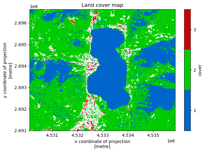
Mapping for each location in space the most often observed semantic concept over time.
[9]:
recipe = sq.QueryRecipe()

recipe["land_cover"] = sq.collection(sq.entity("water"), sq.entity("vegetation"), sq.entity("builtup")).\
    compose().\
    reduce("mode", "time")

response = recipe.execute(**context)
[10]:
f, ax = plt.subplots(1, figsize = (7, 5))

land_cover = response["land_cover"]
values = [1, 2, 3]
levels = [x - 0.5 for x in values + [max(values) + 1]]
colors = ["#0066CC", "#00CC00", "#CC0000"]
land_cover.plot(ax = ax, levels = levels, colors = colors, cbar_kwargs = {"ticks": values, "label": "cover"})
ax.set_title("Land cover map")

plt.tight_layout()
plt.draw()
Cloud and snow cover maps#
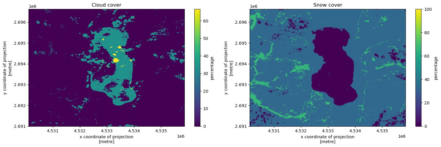
Mapping for each location in space the percentages of times respectively cloud and snow were observed there.
[11]:
recipe = sq.QueryRecipe()

recipe["cloud_cover"] = sq.entity("cloud").\
    reduce("percentage", "time")

recipe["snow_cover"] = sq.entity("snow").\
    reduce("percentage", "time")

response = recipe.execute(**context)
[12]:
f, (ax1, ax2) = plt.subplots(1, 2, figsize = (15, 5))

cloud_cover = response["cloud_cover"]
cloud_cover.plot(ax = ax1, cbar_kwargs = {"label": "percentage"})
ax1.set_title("Cloud cover")

snow_cover = response["snow_cover"]
snow_cover.plot(ax = ax2, cbar_kwargs = {"label": "percentage"})
ax2.set_title("Snow cover")

plt.tight_layout()
plt.draw()
Semantic content based image retrieval#
Check for each image if it has a cloud cover less than 10 percent.
[13]:
recipe = sq.QueryRecipe()

recipe["cloud_free_images"] = sq.entity("cloud").\
    reduce("percentage", "space").\
    evaluate("less", 10)

response = recipe.execute(**context)
[14]:
response["cloud_free_images"].astype("bool").sq.to_dataframe()
[14]:
| cloud_free_images | |
|---|---|
| time | |
| 2019-12-15 10:17:33.408715 | False |
| 2020-09-05 10:17:43.167942 | True |
| 2020-12-19 10:17:34.610661 | True |
Parcel statistics#
Using a spatial extent that consists of multiple non-overlapping spatial features, calculate the average water count over time per spatial feature.
[15]:
parcels = sq.SpatialExtent(gpd.read_file("files/parcels.geojson"))
[16]:
parcels.features.to_crs(4326).explore()
[16]:
[17]:
new_context = copy.deepcopy(context)
new_context["space"] = parcels
[18]:
recipe = sq.QueryRecipe()

recipe["avg_water_count_per_parcel"] = sq.entity("water").\
    reduce("count", "time").\
    groupby(sq.self().extract("space", "feature")).\
    reduce("mean", "space").\
    concatenate("parcel")

response = recipe.execute(**new_context)
[19]:
df = response["avg_water_count_per_parcel"].sq.to_dataframe()
df
[19]:
| avg_water_count_per_parcel | |
|---|---|
| parcel | |
| Northern | 0.939145 |
| Southern | 1.175439 |
Seasonal aggregates#
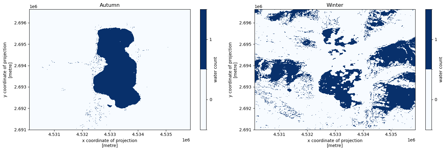
We create a water count map for each season in the data separately. We use the built-in “season” component of the time dimension, which defines seasons as: 1 = March, April, May; 2 = June, July, August; 3 = September, October, November; 4 = December, January, February.
[20]:
recipe = sq.QueryRecipe()

recipe["water_count_per_season"] = sq.entity("water").\
    groupby(sq.self().extract("time", "season")).\
    reduce("count", "time").\
    concatenate("season")

response = recipe.execute(**context)
[21]:
f, (ax1, ax2) = plt.subplots(1, 2, figsize = (15, 5))

water_count_per_season = response["water_count_per_season"]
values = list(range(int(np.nanmin(water_count_per_season)), int(np.nanmax(water_count_per_season)) + 1))
levels = [x - 0.5 for x in values + [max(values) + 1]]
colors = plt.cm.Blues

autumn = water_count_per_season.sel(season = "September, October, November")
autumn.plot(ax = ax1, levels = levels, cmap = colors, cbar_kwargs = {"ticks": values, "label": "water count"})
ax1.set_title("Autumn")

winter = water_count_per_season.sel(season = "December, January, February")
winter.plot(ax = ax2, levels = levels, cmap = colors, cbar_kwargs = {"ticks": values, "label": "water count"})
ax2.set_title("Winter")

plt.tight_layout()
plt.draw()
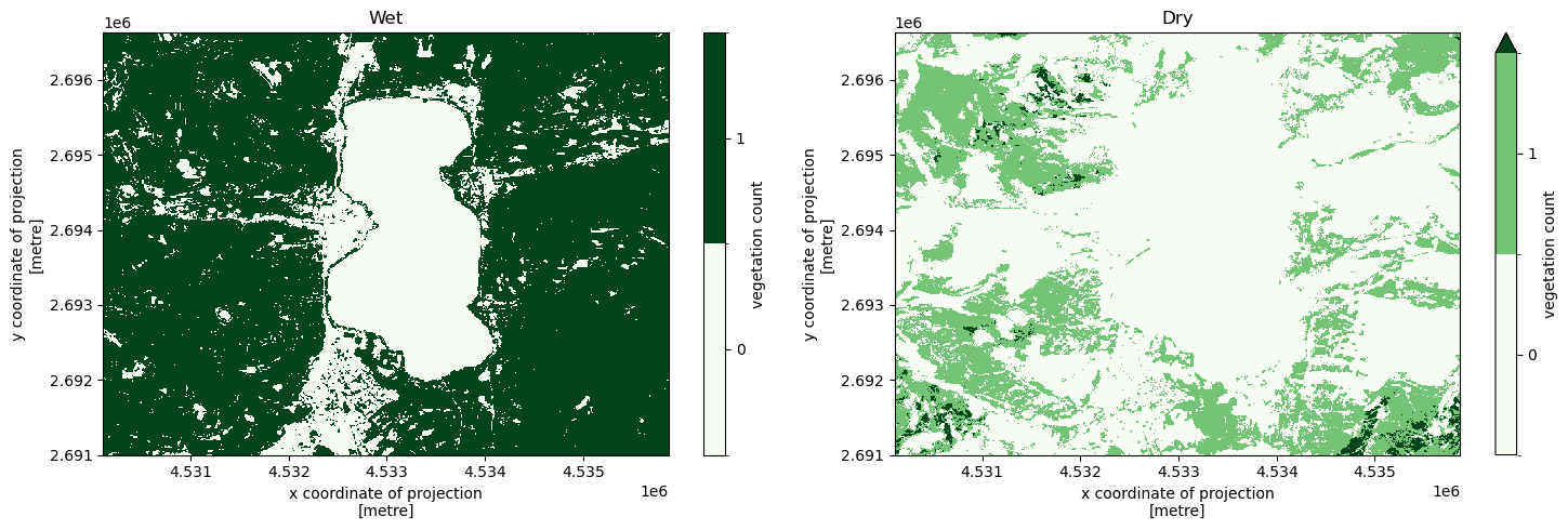
We can do the same with self-defined custom seasons. Conceptually it may even make sense to store such season definitions as being “temporal entities” in the mapping, such that they can easily be re-used in different results. This can be achieved by starting the rules of the entity with a self reference, such that they are applied to the active evaluation object whenever referenced in a query recipe.
Let’s define a imaginary “wet” and “dry” seasons and compute seasonal vegetation counts for them.
[22]:
newmapping = copy.deepcopy(mapping)
newmapping["entity"]["wet_season"] = {"period": sq.self().extract("time", "month").evaluate("in", sq.interval(6, 11))}
newmapping["entity"]["dry_season"] = {"period": sq.self().extract("time", "month").evaluate("not_in", sq.interval(6, 11))}
[23]:
newcontext = copy.deepcopy(context)
newcontext["mapping"] = newmapping
[24]:
recipe = sq.QueryRecipe()

recipe["vegetation_count_per_season"] = sq.entity("vegetation").\
    groupby(sq.collection(sq.entity("wet_season"), sq.entity("dry_season")).compose()).\
    reduce("count", "time").\
    concatenate("season")

response = recipe.execute(**newcontext)
[25]:
f, (ax1, ax2) = plt.subplots(1, 2, figsize = (15, 5))

vegetation_count_per_season = response["vegetation_count_per_season"]
values = list(range(int(np.nanmin(water_count_per_season)), int(np.nanmax(water_count_per_season)) + 1))
levels = [x - 0.5 for x in values + [max(values) + 1]]
colors = plt.cm.Greens

autumn = vegetation_count_per_season.sel(season = "wet_season")
autumn.plot(ax = ax1, levels = levels, cmap = colors, cbar_kwargs = {"ticks": values, "label": "vegetation count"})
ax1.set_title("Wet")

winter = vegetation_count_per_season.sel(season = "dry_season")
winter.plot(ax = ax2, levels = levels, cmap = colors, cbar_kwargs = {"ticks": values, "label": "vegetation count"})
ax2.set_title("Dry")

plt.tight_layout()
plt.draw()
Time of first vegetation observation#
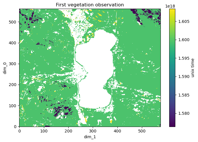
Find for each spatial pixel at which timestamp vegetation was first observed.
[26]:
recipe = sq.QueryRecipe()

recipe["dates"] = sq.entity("vegetation").\
    filter(sq.self()).\
    assign_time().\
    reduce("first", "time")

response = recipe.execute(**context)
[27]:
f, ax = plt.subplots(1, figsize = (7, 5))

dates = xr.DataArray(np.where(np.isfinite(response["dates"]), response["dates"].astype(float), np.nan))
dates.plot(ax = ax, cbar_kwargs = {"label": "unix time"})
ax.set_title("First vegetation observation")

plt.tight_layout()
plt.draw()
